Plot 3D
Fig. 24 shows a typical view of the 3D tab for 3D visualizations of the magnitude frequency response and poles / zeros. Fig. 24 is a surface plot which looks nice but takes the longest time to compute.
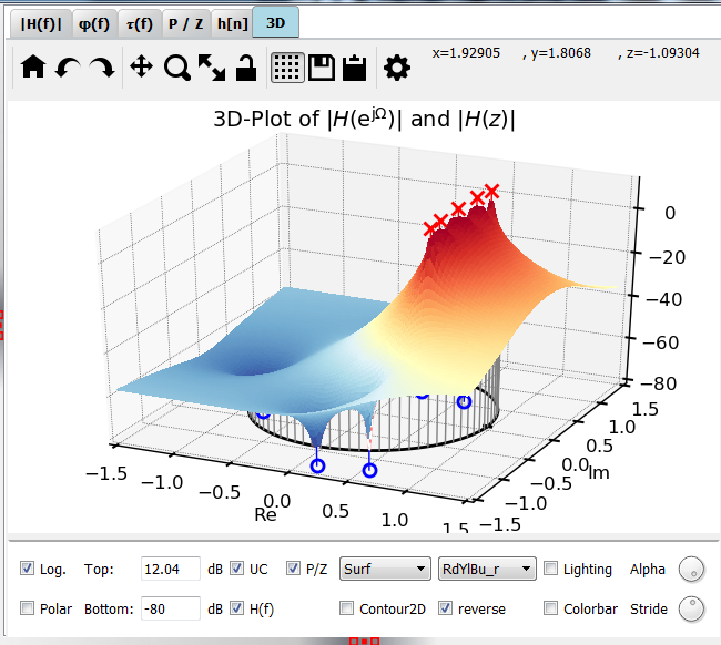
Fig. 24 Screenshot of the 3D tab (surface plot)
You can plot 3D visualizations of \(|H(z)|\) as well as \(|H(e^{j\omega})|\) along the unit circle (UC).
For faster visualizations, start with a mesh plot (Fig. 25) or a contour plot and switch to a surface plot when you are pleased with scale and view.
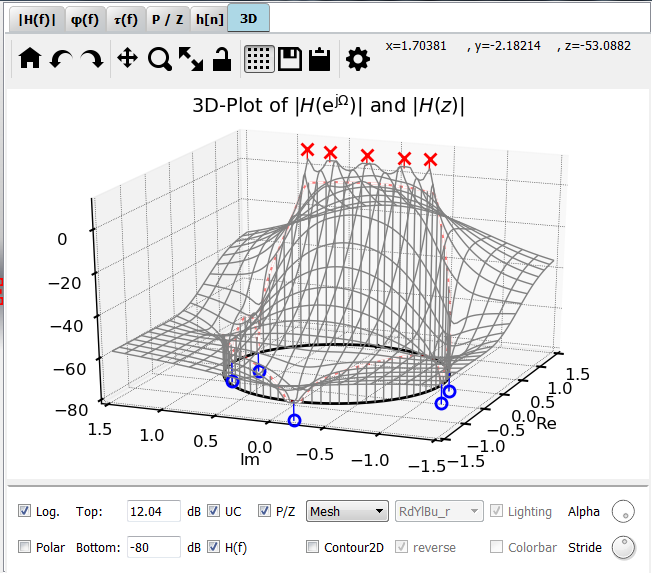
Fig. 25 Screenshot of the 3D tab (mesh plot)